



TL;DR
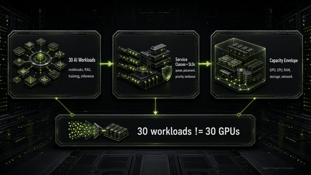
An expected workload count is not a GPU requirement. Thirty concurrent notebooks, RAG services, inference endpoints, fine-tuning jobs, or distributed training runs can create radically different demands for GPU memory, accelerator time, CPU, system memory, storage throughput, metadata operations, network bandwidth, scheduling policy, and failure reserve.
Capacity planning should begin by defining workload service classes and service-level objectives. For each class, measure arrival rate, runtime, queue tolerance, completion-time objective, GPU memory footprint, compute intensity, allocation model, cold-start behavior, and supporting infrastructure demand. Then calculate both a service-capacity floor and a placement-capacity floor. The larger floor governs the design.
In the worked model in this article, three mixes each contain 30 concurrently running workloads. After applying explicit placement rules, utilization targets, 20 percent growth, eight-GPU node rounding, and one-node N+1 reserve, the estimated installed capacity ranges from 24 GPUs to 144 GPUs. The workload count never changed. The service envelope did.
Introduction
Architects are often asked a deceptively simple question: “How many AI workloads can this GPU platform support?” The question usually arrives before anyone has defined what a workload is, how long it runs, whether it can wait, how much GPU memory it consumes, whether it needs a whole GPU, or what happens when a node is unavailable.
That is how GPU capacity planning turns into procurement arithmetic. Someone estimates 30 workloads, assumes some sharing ratio, divides by the number of GPUs in a node, and adds a small percentage for growth. The result looks precise, but it is built on an undefined unit.
A notebook with an idle Python kernel is not equivalent to an eight-GPU training job. A retrieval-augmented generation application is not one indivisible GPU workload. An online inference endpoint with a strict tail-latency objective cannot be treated like a checkpointable batch job. Even two deployments of the same model can have different capacity envelopes because context length, batching, quantization, model-loading behavior, data pipelines, and concurrency are different.
The better architectural position is straightforward:
Capacity planning must start with workload service classes and SLOs, not with a target GPU count.
This article develops that position into a reusable sizing method. It combines workload profiling, GPU-memory placement, queueing, utilization headroom, supporting infrastructure, and failure-domain reserves. It also provides a worked 30-workload model to show why a single concurrency number cannot produce a defensible GPU design.
The Architectural Mistake Is Counting Workloads Instead of Defining Service
A workload count tells an architect how many logical activities are expected. It does not reveal how much useful work must be completed, how quickly it must finish, or which resources must be available at the same time.
Consider the difference between these requests:
- Support 30 data-science notebooks during business hours.
- Support 30 online inference replicas with strict latency objectives.
- Support 30 fine-tuning and distributed-training jobs that must all run simultaneously.
- Accept 30 submitted jobs, but allow 20 of them to wait in a controlled queue.
All four statements use the number 30. None describe the same platform.
The NVIDIA developer-forum discussion supplied with this assignment illustrates another reason raw GPU metrics can mislead. In that case, one multi-stream process and several single-stream processes produced very different utilization and throughput behavior. NVIDIA staff pointed toward the upstream video-decoding and feed path as a possible bottleneck and recommended deeper telemetry. The case is not a universal benchmark, but it demonstrates a useful operational lesson: process count, stream count, and reported GPU utilization do not automatically equal useful application throughput [11].
Vendor-validated fact: NVIDIA Run:ai positions dynamic allocation, policy-driven governance, workload orchestration, quotas, priority, and scheduling as mechanisms for improving how shared accelerator capacity is consumed [1], [2].
Architectural interpretation: A scheduler can redistribute and govern capacity, but it cannot turn an undefined workload into a reliable sizing unit. The platform still needs workload profiles, service classes, and measured demand.
A Workload Is a Service Envelope, Not a GPU Number
A defensible workload definition has two parts: a resource envelope and a service envelope.
The resource envelope
The resource envelope describes what the workload consumes while it is admitted and running:
- GPU count or fractional allocation
- GPU memory, including model weights, KV cache, activations, framework overhead, and margin
- CPU cores and CPU scheduling sensitivity
- system memory and page-cache demand
- storage read throughput, write throughput, IOPS, and metadata activity
- east-west, north-south, and storage-network traffic
- local scratch and persistent-capacity requirements
- topology, affinity, and gang-scheduling constraints
The service envelope
The service envelope describes how the platform is expected to deliver that capacity:
- arrival pattern and active concurrency
- acceptable queue time
- completion-time objective
- latency or throughput objective
- guaranteed or burst treatment
- priority and preemption policy
- cold-start tolerance
- retry and checkpoint behavior
- maintenance and failure behavior
- growth horizon
The capacity-planning flow should therefore look like this:
The important point is that installed GPU count appears at the end of the process. It is an output, not the starting assumption.
Build Workload Profiles Before You Size Hardware
The following table is a reusable first-pass classification. It does not assign universal resource values. It identifies the dominant questions that must be measured for each workload family.
| Workload profile | Dominant capacity question | Common placement posture | Supporting-resource pressure | Queue and SLO posture |
|---|---|---|---|---|
| Interactive notebooks | How much GPU memory remains resident while compute is intermittent? | Fractional, MIG, time-sliced, or whole GPU for isolation-sensitive work | CPU kernels, data loading, package environments, shared-file metadata, idle memory | Usually guaranteed access with bounded startup time, but not guaranteed continuous GPU compute |
| Full training | How many GPUs must operate together, and how efficiently do they scale? | Whole GPU, multi-GPU, gang-scheduled, topology-aware | Sustained dataset reads, checkpoint writes, CPU preprocessing, high-speed east-west networking | Often queue tolerant, but completion-time and checkpoint-recovery objectives matter |
| Fine-tuning | Does the method fit on one GPU, or does optimizer and model state force multi-GPU placement? | Whole GPU or multi-GPU; low-rank adaptation may fit smaller allocations | Dataset reads, checkpointing, CPU tokenization, host-memory staging | Usually burst or scheduled service, with deadlines rather than request latency |
| Embeddings | Is throughput limited by GPU compute, tokenization, storage feed, or batching? | Fractional, time-sliced, MIG, or dedicated accelerator at high volume | CPU tokenization, document reads, write path to vector storage | Highly batchable and commonly queue tolerant |
| RAG | Which stages use GPU, and which use CPU, memory, metadata, search, and network? | Split retrieval, reranking, and generation into separate profiles | Vector index latency, metadata filters, document access, CPU memory, network hops | Online RAG needs end-to-end latency SLOs; ingestion is usually batch-oriented |
| Batch inference | What throughput must be completed by a deadline? | Fractional or whole GPU, high batching, often preemptible | Model loading, input/output storage, CPU preprocessing | Queue tolerant if deadline and restart behavior are explicit |
| Online inference | What replica count protects tail latency and availability during bursts or failures? | Warm, reserved, non-preemptible or tightly controlled sharing | Model load, KV cache, request networking, tokenization, telemetry | Near-zero queue tolerance, tail-latency SLO, availability reserve, controlled rollout |
This classification exposes several common mistakes.
A RAG application should not be sized as “one GPU workload.” Retrieval, reranking, prompt assembly, model inference, and response streaming have different resource patterns. A notebook should not be considered free merely because its GPU compute utilization is low. It may hold enough GPU memory to block another placement. An eight-GPU training job is not eight independent one-GPU jobs because all eight devices may need to be available together in a suitable topology.
GPU Memory Is Often the First Placement Constraint
GPU compute averages are useful for service-capacity planning, but GPU memory often decides whether a workload can be placed at all.
A practical placement estimate begins with:
Required GPU memory = model weights
                    + KV cache
                    + activations and working buffers
                    + framework and runtime overhead
                    + operational safety margin
Vendor-validated fact: NVIDIA NIM evaluates model profiles against available VRAM using model weights, KV cache, activation estimates, and runtime overhead. Profiles that exceed available VRAM are excluded, and reducing maximum context length can reduce memory pressure when weights fit but the full context allocation does not [5].
Aggregate memory is not enough
Worked example: Assume six independent model services each require 45 GB of GPU memory and the platform uses 80 GB GPUs.
A simplistic aggregate calculation says:
6 workloads x 45 GB = 270 GB
270 GB / 80 GB per GPU = 3.375 GPUs
Round up = 4 GPUs
That result is impossible to place because two 45 GB models do not fit on one 80 GB GPU. The actual placement floor is six GPUs, not four.
This is why a capacity model needs bin-packing logic or trace-based placement simulation. Total VRAM divided by GPU memory is not a sufficient sizing method.
Context length and concurrency change the memory envelope
Online inference memory is not only model-weight memory. KV cache grows with context length, batch size, concurrent sequences, model architecture, and data type. A model that fits during a single-user test may fail or shed throughput when concurrency rises. The workload profile should therefore record both a minimum memory footprint and a concurrency-dependent memory curve.
Memory fragmentation creates stranded capacity
A cluster can report free GPU memory in aggregate and still be unable to start a job. Common reasons include:
- free memory is split across GPUs that cannot satisfy one placement
- a MIG geometry does not provide the requested slice shape
- a gang-scheduled workload cannot find enough GPUs on the same node or topology island
- time-sliced workloads share compute but have no separate memory pool
- resident notebook or inference processes hold memory while doing little compute
The scheduler needs placement-aware metrics, not merely fleet-wide averages.
Choose the GPU Allocation Model Explicitly
Whole-GPU, MIG, time-sliced, and scheduler-managed fractional allocation are not interchangeable. Each makes a different promise about isolation, memory, oversubscription, observability, and failure behavior.
| Allocation model | What is allocated | Isolation posture | Oversubscription | Best fit | Capacity-planning caution |
|---|---|---|---|---|---|
| Whole GPU | One or more complete physical GPUs | Strongest operational separation of the listed options | No | Training, large fine-tunes, sensitive inference, predictable performance | Lower density for bursty or small workloads; topology and gang placement remain important |
| MIG | Hardware-partitioned GPU instances on supported GPUs | Dedicated memory and compute partitions within supported geometry | No compute oversubscription inside a slice | Predictable small or medium workloads needing stronger isolation | Fixed profiles can strand capacity; profile changes are maintenance events and may require workloads to stop [3] |
| Time-slicing | Multiple processes or pods take turns on the same GPU | No separate memory or fault isolation between replicas | Yes | Trusted, bursty, compute-light workloads that tolerate interference | Replica count is not a guaranteed compute share; telemetry attribution can be weaker [4] |
| Shared or fractional scheduler allocation | A logical fraction or policy-controlled share, implementation dependent | Depends on the underlying sharing mechanism | Often | Notebooks, embeddings, development, selected inference | A scheduler fraction is not automatically a hard performance or memory boundary; benchmark the actual runtime path |
Vendor-validated fact: NVIDIA documents MIG as hardware partitioning with isolated GPU instances on supported accelerators. Reconfiguration can require workload eviction, GPU-pod shutdown, node cordoning, or reboot depending on the platform state [3].
Vendor-validated fact: NVIDIA documents time-slicing as GPU oversubscription. Time-sliced replicas do not receive memory or fault isolation, and requesting more replicas does not guarantee a proportionally larger compute share [4].
Architectural implication: The allocation model must be a field in the workload profile. An architect cannot apply one cluster-wide “four workloads per GPU” ratio to a platform that mixes whole-GPU training, MIG-backed inference, time-sliced notebooks, and scheduler-managed fractions.
Capacity Comes From Queueing and SLOs
Concurrency is a state, not a demand model. The platform must distinguish between submitted workloads, runnable workloads, running workloads, warm services, cold-starting workloads, and queued work.
Use Little’s Law to estimate average active demand
For a stable workload class:
Average active concurrency (L) = arrival rate (lambda) x average time in system (W)
Little’s Law provides a useful first-order relationship between arrivals, time, and average concurrency [12].
Worked example: A platform receives 24 batch jobs per day, and each job spends an average of four hours from admission to completion.
Arrival rate = 24 jobs / 24 hours = 1 job per hour
Average time in system = 4 hours
Average concurrency = 1 x 4 = 4 jobs
The average is four, but that does not prove four execution slots are enough. If all 24 jobs arrive at 9:00 a.m., the queue-time distribution will be very different from a uniform arrival pattern. Architects should use observed traces, time-of-day distributions, or simulation when burst shape matters.
Running and queued workloads are different capacity promises
A platform can support 30 submitted workloads while running only 10. That can be a valid design when the queue-time and completion-time objectives are explicit. It is a failed design when stakeholders believe all 30 are guaranteed to start immediately.
Define guaranteed and burst service classes
The following is an example architecture pattern, not a vendor default.
| Example service class | Typical workloads | Capacity promise | Queue objective | Preemption posture | Reserve implication |
|---|---|---|---|---|---|
| Guaranteed real-time | Online inference and latency-sensitive APIs | Warm replicas and protected minimum capacity | Near zero under the stated load envelope | Normally non-preemptible | Reserve for burst, rollout, and failure without violating tail latency |
| Guaranteed interactive | Notebooks, interactive RAG development, engineering tools | Minimum quota with bounded startup | P95 startup or queue measured in minutes | Selected sessions may be reclaimable after idleness | Keep enough placement capacity for business-hour bursts |
| Burst production | Embeddings, batch inference, scheduled fine-tuning | Runs when guaranteed capacity is unused or within assigned burst quota | P95 queue measured in tens of minutes | Checkpointable and preemptible where supported | Use queue depth to absorb short demand spikes |
| Opportunistic research | Exploratory training and long-running experiments | No immediate-start guarantee | Hours may be acceptable | Preemptible with checkpoint and restart controls | Consumes otherwise idle capacity but must not become an availability dependency |
Queue-time and completion-time objectives should be separate:
Queue time       = workload start time - submission time
Completion time  = successful finish time - submission time
Completion time includes queueing, image pull, storage mount, model loading, engine compilation, warm-up, execution, retries, checkpoint recovery, and final output handling. A workload can meet runtime expectations and still miss its completion SLO because the platform ignored queueing or cold start.
Why 100 Percent Sustained Utilization Is Unsafe
A capacity plan built for 100 percent sustained accelerator utilization has no room for burst absorption, maintenance, failure, model reloads, priority inversions, or measurement error. It also assumes that every reported utilization point corresponds to useful work, which is not true.
Vendor-validated fact: NVIDIA defines reported GPU utilization as the percentage of the sampling period during which one or more kernels executed. Memory utilization is based on time spent reading or writing device memory [10]. Those measurements are useful, but they do not directly report request latency, samples per second, tokens per second, queue delay, or business completion time.
Queue delay also grows nonlinearly as a shared resource approaches saturation. The following M/M/1 table is an illustrative teaching model, not a prediction of a real AI platform. Actual AI arrivals and service times are more complex.
| Utilization assumption | Illustrative mean response-time multiplier |
|---|---|
| 50% | 2.0x service time |
| 70% | 3.3x service time |
| 80% | 5.0x service time |
| 90% | 10.0x service time |
| 95% | 20.0x service time |
The design lesson is not that every cluster should use one universal percentage. The lesson is that capacity targets must be tied to service behavior.
Example planning bands:
- Latency-sensitive online inference: 50 to 65 percent steady-state capacity use.
- Mixed interactive and production services: 60 to 75 percent.
- Checkpointable batch and training pools: 70 to 85 percent when queueing is intentional.
These are planning assumptions for initial modeling, not NVIDIA limits and not substitute benchmarks. A mature platform should replace them with measured utilization-to-SLO curves for its own workload classes.
CPU, System Memory, Storage, and Network Can Set the Real Limit
A GPU platform can have free accelerator capacity and still be unable to deliver more useful work. The limiting resource may be CPU preprocessing, host memory, storage metadata, checkpoint bandwidth, model-loading fan-out, or network collectives.
CPU and system-memory ratios are workload-specific
Avoid one universal ratio such as “eight CPU cores per GPU.” CPU demand changes with tokenization, data decoding, augmentation, serialization, retrieval, orchestration, networking, and runtime implementation. Host memory demand changes with dataset caching, model staging, CPU offload, asynchronous checkpointing, page cache, and vector-search behavior.
A useful workload profile records:
| Supporting resource | Measurement to capture | Why it matters |
|---|---|---|
| CPU cores | Average and peak runnable cores, CPU run queue, per-stage CPU time | A GPU can starve while tokenizers, decoders, or data loaders fall behind |
| System memory | Resident set, page cache, pinned memory, offload, checkpoint staging | Host-memory pressure can increase model-load time, paging, and job failure |
| NUMA locality | CPU, memory, NIC, storage, and GPU locality | Poor locality can reduce effective throughput even when aggregate resources look sufficient |
| CPU-only services | Retrieval, metadata, ingestion, orchestration, API gateways | Buying GPU nodes to obtain more CPU and RAM can be an expensive architectural mistake |
Separate CPU-heavy retrieval, ingestion, metadata, and preprocessing pools from GPU nodes when doing so improves economics and failure isolation.
Model loading and cold starts consume real capacity
Cold start can include:
Scale-to-zero can improve idle efficiency, but it converts capacity savings into queue or latency risk. Model-loading traffic can also create a synchronized storage and network burst during scaling, rollout, or recovery.
Vendor-validated fact: NVIDIA describes Model Streamer in Run:ai as using concurrent reads and direct transfer toward GPU memory to reduce model-loading delay [1]. That is a useful optimization pattern, but actual cold-start performance still depends on model format, cache state, storage, network, CPU staging, runtime initialization, and readiness checks.
Capacity reviews should therefore record P50, P95, and P99 duration for each cold-start stage. “GPU available” is not the same as “service ready.”
Storage needs throughput, IOPS, and metadata capacity
Training often needs large sequential reads and burst checkpoint writes. Notebooks and model repositories can create large numbers of file-open, stat, list, and small-file operations. RAG systems can combine vector-index access, metadata filtering, document retrieval, and ingestion writes. Online inference can create model-loading fan-out during recovery or horizontal scaling.
Vendor-validated fact: NVIDIA’s enterprise AI guidance treats parallel scale-out storage, throughput, IOPS, checkpoints, embeddings, and tiered storage as explicit architecture concerns. NVIDIA’s storage guidance also distinguishes the read, write, checkpoint, fine-tuning, inference, and RAG patterns that storage must serve [6], [7].
A reusable storage worksheet should capture:
- aggregate and per-node read throughput
- aggregate and per-node write throughput
- checkpoint size, interval, and completion time
- IOPS and latency distribution
- metadata operations per second
- file and object count
- cache hit rate
- model-load fan-out during scale or recovery
- isolation between training, inference, checkpoints, and control-plane data
Distributed workloads are network-sensitive
Multi-node training and some model-parallel inference designs exchange large amounts of synchronization and collective-communication traffic. Effective performance depends on topology, latency, congestion, oversubscription, NIC placement, and the relationship between GPUs, CPUs, and network interfaces.
Vendor-validated fact: NVIDIA’s AI-factory reference guidance separates high-speed east-west compute communication from north-south, storage, and management traffic. Its HGX topology guidance describes an RDMA-capable leaf-spine compute fabric for scale-out GPU workloads [6], [8].
The capacity question is not only “Do we have enough aggregate network bandwidth?” It is also:
- Can the scheduler place the job within an appropriate topology?
- What collective bandwidth does the job achieve under contention?
- Does storage traffic compete with the compute fabric?
- What happens when one leaf, link, NIC, or rack is unavailable?
- Does adding GPU nodes improve throughput, or move the bottleneck into the fabric?
A Reusable Capacity-Planning Method
The following method separates service demand from placement demand.
Define the variables
| Variable | Meaning |
|---|---|
lambda_i |
Arrival rate for workload class i |
W_i |
Average time in system for class i, including queue and execution when using Little’s Law |
L_i |
Average active concurrency for class i |
g_i |
Measured service GPU equivalent per active workload at the target SLO |
v_i |
GPU-memory and placement requirement for class i |
U_target |
Maximum planned steady-state utilization for the service pool |
r_growth |
Growth reserve over the planning horizon |
G_node |
GPUs per node |
F |
Failure-domain reserve expressed in GPUs or nodes |
Calculate average active concurrency
L_i = lambda_i x W_i
For scheduled waves or bursty arrival patterns, replace the average with trace replay, percentile concurrency, or simulation.
Calculate the service-capacity floor
G_service = ceiling(sum(L_i x g_i) / U_target)
The g_i value is not a requested GPU count. It is the measured accelerator service demand required to meet the workload’s throughput, latency, or completion objective.
Calculate the placement-capacity floor
G_placement = bin-pack(
    GPU memory,
    whole-GPU or partition geometry,
    topology and gang requirements,
    isolation rules,
    affinity and anti-affinity
)
A spreadsheet can approximate this for simple profiles. Mixed MIG geometries, multi-GPU jobs, and time-varying queues usually justify scheduler trace replay or simulation.
Apply the largest resource floor
G_day_one = max(
    G_service,
    G_placement,
    G_topology,
    GPU-equivalent floor implied by CPU,
    GPU-equivalent floor implied by system memory,
    GPU-equivalent floor implied by storage,
    GPU-equivalent floor implied by network
)
Apply growth, node rounding, and resilience
G_growth = ceiling(G_day_one x (1 + r_growth))

G_rounded = round up G_growth to complete GPU nodes

G_installed = G_rounded + failure-domain reserve
Do not assume that one spare GPU equals N+1 when the scheduling and maintenance unit is an eight-GPU node. Do not assume one spare node protects a design whose credible failure domain is a four-node rack or an entire fabric leaf.
Worked Capacity Model for 30 Concurrent Workloads
This model intentionally uses explicit assumptions. It is not an NVIDIA sizing guide, not a hardware benchmark, and not a substitute for measurements from the intended models and datasets.
Platform assumptions
| Planning assumption | Value used in the example |
|---|---|
| GPUs per node | 8 |
| GPU memory | 80 GB per GPU |
| CPU capacity per GPU node | 192 cores |
| System memory per GPU node | 2 TiB |
| Growth reserve | 20% |
| Failure and maintenance reserve | One complete eight-GPU node |
| Development-heavy target utilization | 70% |
| Balanced-enterprise target utilization | 72% |
| Training-heavy target utilization | 78% |
| Failure-domain model | One-node N+1 only; rack and fabric failures evaluated separately |
Per-workload planning assumptions
The GPU-service equivalent represents measured average accelerator demand at the intended service objective. The placement unit represents the allocatable GPU footprint needed to admit the workload. These two values differ because a workload can reserve memory and placement while using less than a full GPU of sustained compute.
| Workload unit | Placement units | Service GPU equivalent | CPU cores | System memory | Storage envelope | Network envelope |
|---|---|---|---|---|---|---|
| Notebook | 0.25 | 0.10 | 4 | 32 GiB | 0.05 GB/s | 1 Gb/s |
| Embeddings worker | 0.25 | 0.20 | 8 | 48 GiB | 0.30 GB/s | 2 Gb/s |
| RAG GPU stage | 0.25 | 0.15 | 8 | 64 GiB | 0.20 GB/s | 2 Gb/s |
| Batch inference worker | 0.50 | 0.35 | 8 | 32 GiB | 0.50 GB/s | 2 Gb/s |
| Online inference replica | 1.00 | 0.70 | 8 | 64 GiB | 0.50 GB/s | 10 Gb/s |
| One-GPU fine-tune | 1.00 | 0.85 | 8 | 128 GiB | 1.00 GB/s | 5 Gb/s |
| Two-GPU fine-tune | 2.00 | 1.70 | 16 | 128 GiB | 2.00 GB/s | 50 Gb/s |
| Four-GPU fine-tune | 4.00 | 3.40 | 32 | 256 GiB | 4.00 GB/s | 100 Gb/s |
| Eight-GPU distributed training | 8.00 | 6.80 | 64 | 512 GiB | 8.00 GB/s | 400 Gb/s |
Assumption boundary: Storage and network values are concurrent design envelopes used to reveal infrastructure pressure. They are not guaranteed wire-rate requirements or vendor benchmark results. Real designs should replace them with observed throughput distributions and topology-specific measurements.
Three mixes with the same workload count
| Workload profile | Development-heavy | Balanced enterprise | Training-heavy |
|---|---|---|---|
| Notebooks | 12 | 6 | 4 |
| Embeddings workers | 6 | 4 | 2 |
| RAG GPU stages | 6 | 4 | 2 |
| Online inference replicas | 0 | 6 | 2 |
| Batch inference workers | 4 | 4 | 4 |
| One-GPU fine-tunes | 2 | 0 | 0 |
| Two-GPU fine-tunes | 0 | 4 | 0 |
| Four-GPU fine-tunes | 0 | 0 | 8 |
| Eight-GPU distributed training jobs | 0 | 2 | 8 |
| Total concurrent workloads | 30 | 30 | 30 |
Development-heavy result
Service demand = 6.4 GPU equivalents
Service floor  = ceiling(6.4 / 0.70) = 10 GPUs
Placement floor = 10 GPUs
Day-one floor   = max(10, 10) = 10 GPUs
With 20% growth = ceiling(10 x 1.20) = 12 GPUs
Node rounding   = 16 GPUs across 2 nodes
Add one N+1 node = 24 installed GPUs across 3 nodes
The development-heavy mix is dominated by placement and memory residency rather than sustained compute. It also needs 192 CPU cores, approximately 1.4 TiB of system memory, 7.6 GB/s of aggregate storage envelope, and 54 Gb/s of aggregate network envelope before growth and resilience are applied.
Balanced-enterprise result
Service demand = 28.0 GPU equivalents
Service floor  = ceiling(28.0 / 0.72) = 39 GPUs
Placement floor = ceiling(35.5) = 36 GPUs
Day-one floor   = max(39, 36) = 39 GPUs
With 20% growth = ceiling(39 x 1.20) = 47 GPUs
Node rounding   = 48 GPUs across 6 nodes
Add one N+1 node = 56 installed GPUs across 7 nodes
The balanced mix requires 360 CPU cores, approximately 2.6 TiB of system memory, 31.3 GB/s of storage envelope, and 1,090 Gb/s of concurrent network envelope. Its distributed training and multi-GPU fine-tunes make topology and fabric design material even though most workloads are smaller services.
Training-heavy result
Service demand = 85.5 GPU equivalents
Service floor  = ceiling(85.5 / 0.78) = 110 GPUs
Placement floor = 102 GPUs
Day-one floor   = max(110, 102) = 110 GPUs
With 20% growth = ceiling(110 x 1.20) = 132 GPUs
Node rounding   = 136 GPUs across 17 nodes
Add one N+1 node = 144 installed GPUs across 18 nodes
The training-heavy mix requires 864 CPU cores, approximately 6.6 TiB of system memory, 100.2 GB/s of storage envelope, and 4,040 Gb/s of concurrent network envelope. GPU count drives the node total, but the platform would still fail if storage checkpoints or collective communication cannot sustain the jobs.
The same 30 workloads produce three different platforms
| Result | Development-heavy | Balanced enterprise | Training-heavy |
|---|---|---|---|
| Concurrent workload count | 30 | 30 | 30 |
| Day-one GPU floor | 10 | 39 | 110 |
| GPUs after growth and node rounding | 16 | 48 | 136 |
| GPUs with one-node N+1 | 24 | 56 | 144 |
| Installed GPU nodes | 3 | 7 | 18 |
| CPU demand before growth | 192 cores | 360 cores | 864 cores |
| System-memory demand before growth | 1.4 TiB | 2.6 TiB | 6.6 TiB |
| Storage design envelope | 7.6 GB/s | 31.3 GB/s | 100.2 GB/s |
| Network design envelope | 54 Gb/s | 1,090 Gb/s | 4,040 Gb/s |
This is the central result: the same concurrency statement produces an installed estimate of 24, 56, or 144 GPUs. The difference comes from workload mix, allocation assumptions, SLOs, placement, topology, utilization target, node size, growth, and failure reserve.
A procurement request that contains only “30 concurrent AI workloads” is therefore not ready for hardware selection.
Maintenance, Growth, and Failure Reserves Must Be Separate Decisions
A reserve is useful only when its purpose is explicit.
Growth reserve
Growth reserve covers forecast demand over the planning horizon. Once growth arrives, that capacity is no longer spare. It cannot also be counted as failure reserve.
Maintenance reserve
Maintenance reserve covers planned node drain, driver updates, firmware changes, MIG reconfiguration, platform upgrades, and other lifecycle work. MIG profile changes can be disruptive because GPU workloads may need to stop before geometry changes [3].
Hardware-failure reserve
Hardware reserve covers the largest failure event the service is designed to survive while still meeting guaranteed SLOs. This may be:
- one GPU
- one complete GPU node
- one rack or chassis
- one fabric leaf or network plane
- one power domain
- one availability zone or site
Why N+1 may be too small
In the worked example, N+1 means one additional eight-GPU node. That protects against one node being unavailable, assuming the surviving nodes can satisfy topology and placement constraints.
It does not automatically protect against:
- losing a rack containing four GPU nodes
- losing a shared top-of-rack switch
- a storage outage that affects every node
- a scheduler or control-plane failure
- a multi-node job that cannot be reshaped after one node fails
- an upgrade that temporarily affects more than one node or capacity pool
For larger failure domains, calculate reserve from the largest credible concurrent loss and the workloads that must remain guaranteed. Some burst and opportunistic classes may queue during a failure, while real-time inference and committed training windows may require protected capacity.
Measure Real Demand Before Purchasing the Next GPU Node
The next GPU node should be purchased because measured service demand exceeds a defined threshold, not because one dashboard shows high utilization.
Vendor-validated fact: NVIDIA DCGM Exporter exposes GPU telemetry for Prometheus and Kubernetes-oriented monitoring [9]. This is a useful foundation, but GPU metrics must be correlated with scheduler, storage, network, and application evidence.
A practical evidence pack should include:
| Evidence domain | Measurements to retain | Decision it supports |
|---|---|---|
| Scheduler | Arrival rate, requested resources, actual runtime, P50/P95/P99 queue time, pending reason, preemption, quota use, placement failures | Whether unmet demand is real, which service class is affected, and whether the problem is policy or capacity |
| GPU | SM and tensor activity, framebuffer use, memory bandwidth, power, clocks, PCIe or interconnect activity | Whether the GPU is compute-bound, memory-bound, stalled, underfed, or fragmented |
| Application | Tokens/s, requests/s, samples/s, P95/P99 latency, batch efficiency, completion time, error rate | Whether useful work and SLOs improve with more accelerator capacity |
| CPU and memory | CPU run queue, per-stage CPU time, NUMA locality, page faults, pinned memory, cache use | Whether supporting compute is starving the accelerator |
| Storage | Read and write throughput, latency, IOPS, metadata operations, checkpoint duration, cache hit rate | Whether data, model loading, vector access, or checkpoints are limiting throughput |
| Network | Collective bandwidth, congestion, retransmits, oversubscription, link balance, cross-rack traffic | Whether distributed scaling is limited by topology or fabric capacity |
| Cold start | Image pull, mount, model transfer, compile, warm-up, readiness | Whether scaling and recovery can meet service objectives |
Before approving another node, answer these questions:
- Which workload class is missing its queue-time, latency, throughput, or completion SLO?
- Is the active constraint service compute, GPU memory, topology, CPU, system memory, storage, network, or policy?
- Are workloads pending because capacity is unavailable, or because requests and limits are poorly specified?
- Would repacking, quota changes, checkpointing, batching, model quantization, context reduction, or pipeline optimization recover enough capacity?
- Can the platform absorb the next credible failure after the proposed expansion?
- Will adding nodes create a new bottleneck in storage, network, licensing, power, cooling, or operations?
A high GPU-utilization number can be healthy when useful throughput is strong and queues remain within SLO. A lower utilization number can be unhealthy when workloads are starved by CPU, storage, network, or serial application logic.
Know When to Scale Up and When to Scale Out
Scale-up and scale-out solve different constraints.
| Trigger | Prefer scale-up when | Prefer scale-out when |
|---|---|---|
| Model fit | A model, KV cache, or training state cannot fit on the current GPU or node | Models fit, but more independent replicas or jobs are needed |
| Topology | Workloads require more GPUs in one high-bandwidth topology island | Workloads are independent or scale efficiently across nodes |
| Queue SLO | A single job is too slow even when it starts immediately | Too many jobs or replicas are waiting for placement |
| Online inference | One replica needs a larger accelerator or more local memory | More replicas are needed for throughput, availability, or geographic distribution |
| Training | Intra-node bandwidth and larger local GPU domains improve scaling | Multi-node scaling is efficient and the fabric can support it |
| CPU, RAM, and local NVMe | Per-node supporting resources are the binding constraint | Aggregate supporting resources and parallelism are the constraint |
| Failure-domain design | Larger nodes reduce coordination but increase loss per failure | More nodes improve distribution, provided the scheduler and fabric handle the complexity |
Scale up when the workload cannot fit or cannot complete efficiently within the current node boundary. Scale out when independent service demand, queue depth, availability, or aggregate throughput exceeds the current fleet.
Do neither until the active bottleneck is verified. Adding GPUs to a storage-bound training pipeline or CPU-bound inference service increases cost without increasing useful work.
A Practical Capacity Review Checklist
Before signing off a GPU-platform capacity plan, confirm that the architecture can answer each of the following:
- Every workload is assigned to a profile and service class.
- Queue-time, completion-time, latency, or throughput objectives are explicit.
- Guaranteed, burst, and opportunistic capacity are separated.
- GPU memory is modeled with weights, cache, activations, runtime overhead, and margin.
- Whole-GPU, MIG, time-sliced, and fractional assumptions are documented.
- Placement is tested for fragmentation, topology, and gang scheduling.
- CPU, system memory, storage, and network requirements are measured per workload class.
- Cold-start stages and model-loading fan-out are measured.
- Utilization targets are derived from SLO behavior rather than a desire to reach 100 percent.
- Growth, maintenance, and failure reserves are not double-counted.
- The reserve protects the intended failure domain, not merely one arbitrary component.
- Scheduler and application telemetry can identify why workloads wait or underperform.
- Scale-up and scale-out triggers are agreed before procurement.
- The model is rerun with real workload traces before the next node purchase.
Conclusion
The question “How many AI workloads can my GPU platform support?” cannot be answered with a workload count alone. A workload becomes a capacity-planning unit only after the architect defines its resource envelope, service envelope, placement constraints, and failure behavior.
The practical method is to classify workloads, assign service classes, model arrivals and duration, calculate both service and placement floors, and then test CPU, memory, storage, network, cold-start, topology, and resilience constraints. GPU count is the final output of that analysis.
The worked example shows why this discipline matters. Thirty concurrent workloads can translate into 24 installed GPUs in a development-heavy environment, 56 in a balanced enterprise mix, or 144 in a training-heavy design under the stated assumptions. Any of those answers can be reasonable. None can be selected from the number 30.
The next capacity review should therefore begin with traces, workload profiles, queue-time and completion-time SLOs, and explicit service classes. Purchase the next GPU node only after the evidence identifies the limiting resource and shows that the proposed scale-up or scale-out action will improve useful work while preserving operational headroom.
