Skip to content
Close Menu

    Subscribe to Updates

    Get the latest news from tastytech.

    What's Hot

    How AI is changing the vulnerability response timeline

    August 12, 2026

    3 Visual Proofs of the Central Limit Theorem to Build Your Intuition

    August 12, 2026

    The Pentagon signed a $75 million bomb deal so quietly it never even showed up on its own contract list

    August 12, 2026
    Facebook X (Twitter) Instagram
    Facebook X (Twitter) Instagram
    tastytech.intastytech.in
    Subscribe
    • AI News & Trends
    • Tech News
    • AI Tools
    • Business & Startups
    • Guides & Tutorials
    • Tech Reviews
    • Automobiles
    • Gaming
    • movies
    tastytech.intastytech.in
    Home»Business & Startups»3 Visual Proofs of the Central Limit Theorem to Build Your Intuition
    3 Visual Proofs of the Central Limit Theorem to Build Your Intuition
    Business & Startups

    3 Visual Proofs of the Central Limit Theorem to Build Your Intuition

    gvfx00@gmail.comBy gvfx00@gmail.comAugust 12, 2026No Comments4 Mins Read
    Share
    Facebook Twitter LinkedIn Pinterest Email


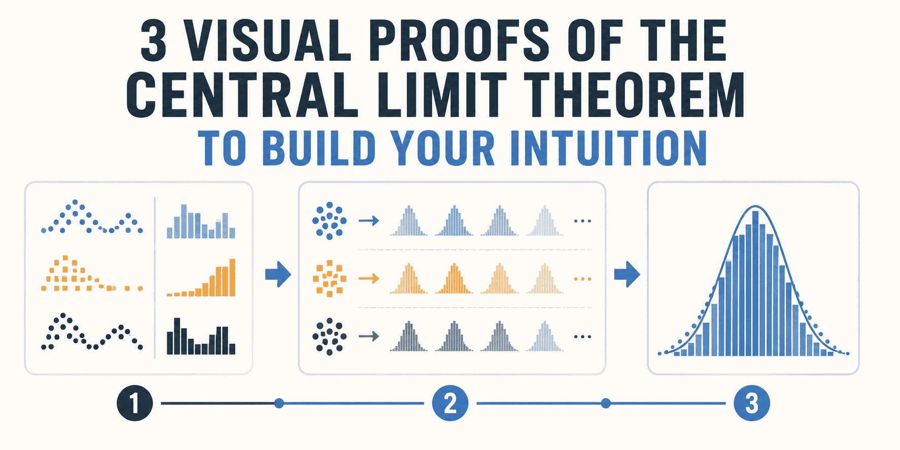
    The central limit theorem (CLT), in very broad terms, tells us that the “magical” bell curve of normal distributions happens (and it does, a lot!) in the real world, often regardless of the data’s original shape. But have you wondered why?

    The bottom line behind CLT is a fundamental statistical rule: if you take enough samples from any data and calculate their averages, these averages will approach a normal distribution — no matter what the original data’s form was.

    To build your intuition, this article shows three visual proofs that the classic bell curve appears in myriad situations.


    Table of Contents

    Toggle
    • # 1. Rolling Multiple Dice
    • # 2. Averaging a Divided Crowd: Bimodal Screen Time
    • # 3. Smoothing Chaotic Skewness: Average Incomes
      • Related posts:
    • 15 Steps to Ensure Your Company's Compliance
    • Is Your Machine Learning Pipeline as Efficient as it Could Be?
    • How to Self-Host n8n on Docker in 5 Simple Steps

    # 1. Rolling Multiple Dice

     
    When rolling a single, six-sided die many times, we intuitively end up with a flat, uniform distribution. However, the story changes when rolling multiple dice simultaneously — for example, five at once. If we calculate the average of those dice results and plot them, a bell curve emerges, peaking around the intermediate scores of 3 and 4. These average scores tend to become much more frequent than those near the extreme values of 1 and 6, which require all dice to score low (or high, respectively): something intuitively more difficult to achieve than having mixed scores compensate each other.

    import numpy as np
    import matplotlib.pyplot as plt
    
    # Simulating 100,000 averages of 5 dice rolls: upper bound of 7 is excluded in randint()
    dice_averages = [np.mean(np.random.randint(1, 7, 5)) for _ in range(100000)]
    
    plt.hist(dice_averages, bins=20, edgecolor="black", color="skyblue")
    plt.title("Distribution of 5-Dice Averages")
    plt.show()


    CLT in action: rolling multiple dice
    Distribution of averages from rolling 5 dice 100,000 times


    # 2. Averaging a Divided Crowd: Bimodal Screen Time

     
    Suppose a video-watching app in which users fall into two sharply distinct categories: they either stay for 1–2 minutes only, or they are “deep scrollers” who stay watching for 30 minutes or more — no users in between. Plotted raw data would, of course, yield a bimodal distribution with a central, deep valley. However, if you repeatedly grab random groups of, say, 40 users, calculate the average screen time, and plot it across many samplings, things change. The distribution of averages utterly ignores the valley between the two peaks and turns into a bell curve.

    # Creating a bimodal distribution (quick checkers and deep scrollers)
    quick = np.random.normal(2, 0.5, 50000)
    deep = np.random.normal(30, 5, 50000)
    bimodal_population = np.concatenate([quick, deep])
    
    # Taking 10,000 samples of 40 users each, and averaging screen times
    screen_time_averages = [np.mean(np.random.choice(bimodal_population, 40)) for _ in range(10000)]
    
    plt.hist(screen_time_averages, bins=30, edgecolor="black", color="mediumpurple")
    plt.title("Averages of Bimodal Screen Times for 10K 40-user samples")
    plt.show()


    CLT in action: averaging bimodal screen times
    Distribution of averages from sampling a bimodal screen time population


    # 3. Smoothing Chaotic Skewness: Average Incomes

     
    Another real-world example of CLT at its finest. Wealth distribution is, let’s face it, remarkably right-skewed, with a vast majority of the population leaning closer to the lower bound. The wealthy minority, therefore, forms a long tail stretching toward the right.

    This picture changes when randomly picking, for instance, 50 people and averaging their incomes. If we repeat this sampling process a few thousand times and plot the averages obtained, the result is — what else could we expect at this point? — a pristine, almost perfectly symmetric bell curve: rich financial outliers get smoothed out by the humbler crowd.

    # Generating heavily skewed "income" data (exponential distribution)
    population = np.random.exponential(scale=50000, size=100000)
    
    # Taking 10,000 samples of 50 people and averaging them
    income_averages = [np.mean(np.random.choice(population, 50)) for _ in range(10000)]
    
    plt.hist(income_averages, bins=30, edgecolor="black", color="salmon")
    plt.title("Averages of Skewed Wealth Samples")
    plt.show()


    CLT in action: averaging skewed income samples
    Distribution of averages from sampling a right-skewed income population


    Iván Palomares Carrascosa is a leader, writer, speaker, and adviser in AI, machine learning, deep learning & LLMs. He trains and guides others in harnessing AI in the real world.

    Related posts:

    My Honest Review on Abacus AI: ChatLLM, DeepAgent & Enterprise

    Object Detection, Pose Estimation & More

    Meet LangSmith Assistant - Polly [An Agent for Agents]

    Share. Facebook Twitter Pinterest LinkedIn Tumblr Email
    Previous ArticleThe Pentagon signed a $75 million bomb deal so quietly it never even showed up on its own contract list
    Next Article How AI is changing the vulnerability response timeline
    gvfx00@gmail.com
    • Website

    Related Posts

    Business & Startups

    The Ultimate Guide to Contributing to Open Source Projects

    August 11, 2026
    Business & Startups

    What is it and How to avoid it

    August 11, 2026
    Business & Startups

    Top 10 AI Influencers of 2026

    August 11, 2026
    Add A Comment
    Leave A Reply Cancel Reply

    Top Posts

    Black Swans in Artificial Intelligence — Dan Rose AI

    October 2, 2025219 Views

    Every Clue That Tony Stark Was Always Doctor Doom

    October 20, 2025143 Views

    We let ChatGPT judge impossible superhero debates — here’s how it ruled

    December 31, 2025109 Views
    Stay In Touch
    • Facebook
    • YouTube
    • TikTok
    • WhatsApp
    • Twitter
    • Instagram

    Subscribe to Updates

    Get the latest tech news from tastytech.

    About Us
    About Us

    TastyTech.in brings you the latest AI, tech news, cybersecurity tips, and gadget insights all in one place. Stay informed, stay secure, and stay ahead with us!

    Most Popular

    Black Swans in Artificial Intelligence — Dan Rose AI

    October 2, 2025219 Views

    Every Clue That Tony Stark Was Always Doctor Doom

    October 20, 2025143 Views

    We let ChatGPT judge impossible superhero debates — here’s how it ruled

    December 31, 2025109 Views

    Subscribe to Updates

    Get the latest news from tastytech.

    Facebook X (Twitter) Instagram Pinterest
    • Homepage
    • About Us
    • Contact Us
    • Privacy Policy
    © 2026 TastyTech. Designed by TastyTech.

    Type above and press Enter to search. Press Esc to cancel.

    Ad Blocker Enabled!
    Ad Blocker Enabled!
    Our website is made possible by displaying online advertisements to our visitors. Please support us by disabling your Ad Blocker.